Welcome to the SolverTable add-in!!
This add-in is a natural extension to the Solver add-in incorporated in
Excel. SolverTable performs sensitivity analysis for an Excel optimization
model, and, in most cases, its output is more relevant and understandable
than the optional sensitivity output provided by Solver itself. SolverTable
is very easy to use, as described below. All it requires is an existing
optimization model. That is, there must be a spreadsheet model already
built, and the corresponding Solver dialog box must already have been filled
out. In this help file, we will explain how to use SolverTable and illustrate
it with several screen shots.
Sections of this Help file
Installing SolverTable
If you clicked on the Help button of the first SolverTable dialog box,
you already installed SolverTable, so you can skip this section.
In general, however, to install SolverTable, copy the SolverTable.xla file
and corresponding help files (SolverTableHelp.htm and the various SolverTable_x.gif
files) to a common directory on your hard drive. Just make sure that all
of the SolverTable files are in the same directory and there
are only alphanumeric characters (no spaces or underscores) in the path
to these files. Then, in Excel, load the add-in with the Tools/Add-ins
menu item. If this is your first time to load SolverTable, you'll need
to click on the Browse button to find the SolverTable.xla file. Otherwise,
there should be a SolverTable item in the list of available add-ins. Just
check its box, and click on OK. SolverTable is no different from any other
Excel add-in; they are all loaded this way. You will know that SolverTable
is loaded when you see a SolverTable menu item under Excel's Data menu.
Uninstalling SolverTable
To uninstall the add-in (remove it from memory), use Excel's Tools/Add-ins
menu item and uncheck the SolverTable box.
An example file
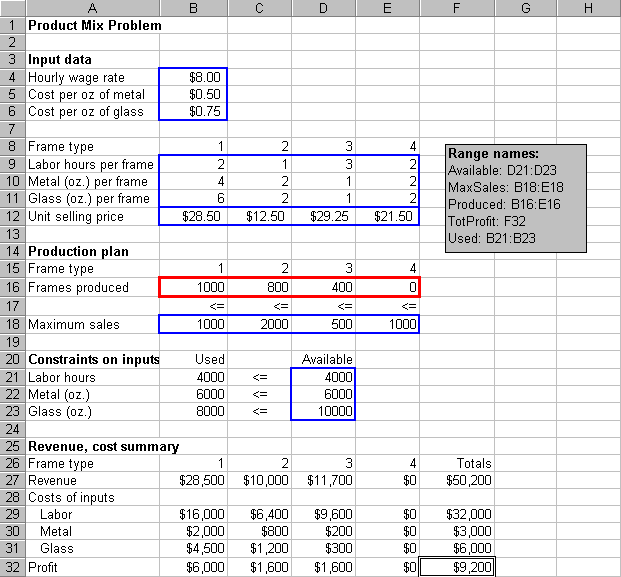
To illustrate SolverTable, we will use the standard product mix model,
a version of which appears in Figure 1. (The conventions we use are that
the inputs are in blue borders, the changing cells are in red borders,
and the objective cell is in a black border.) We assume the Solver dialog
box has already been completed in the obvious way (including checks in
the Assume Linear Model and Assume Non-Negative boxes). Actually, this
model has already been optimized, but this is not necessary for running
SolverTable.

Figure 1
Running SolverTable
The purpose of SolverTable is very much like that of an Excel data table:
to vary one or two inputs and keep track of one or more outputs. The main
difference is that SolverTable runs Solver for each input value (or combination
of input values) and reports the optimal results in the table. Like
data tables, there are essentially two options: one-way tables and two-way
tables, depending on whether there are one or two input cells. However,
unlike Excel data tables, there can be multiple output cells for one-way
and two-way tables. In the latter case, SolverTable creates a separate
table for each output cell. Unfortunately (or fortunately, depending on
your point of view), a table created by SolverTable retains no links to
the original data. If you want to change anything about the table, you'll
have to rerun SolverTable.
Creating a one-way table
To illustrate a one-way table, we'll see how the optimal profit and the
optimal product mix (changing cells) vary as the number of labor hours
available (cell D21) varies from 2000 to 8000 in increments of 1000. Begin
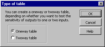
by selecting the Data/SolverTable menu item. This brings up the dialog
box in Figure 2. Fill it out as shown and click on OK.

Figure 2
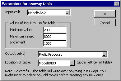
The next dialog box, shown in Figure 3, requires you to specify the
input cell, the input values (which are assumed to be in regular increments),
the output cells, and a location for the table. Note that range names can
be used if they exist. The add-in checks your entries in this dialog box
for "obvious" errors. For example, the input cell should not contain a
formula or a label, the output range should not contain the input cell,
the table location shouldn't write over existing values (unless you say
it is OK to do so), and so on. However, we won't guarantee that it checks
for everything, so be careful when making these entries. Be especially
careful that you choose a location for the table that doesn't write over
any information you don't want to lose (even though you'll be warned if
you try to do so).

Figure 3
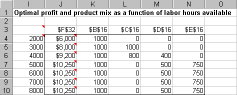
The table itself appears in Figure 4. (We've added the heading in row
1 manually.) The small red triangles are Excel comments that SolverTable
automatically adds to a number of cells. For example, the comment in cell
I4 reminds what the input cell is (in this case, D21). The comments in
column J are the Solver messages you normally see after running Solver.
For this example, they all contain the message you hope to see:
"Solver found a solution. All constraints and optimality conditions are
satisfied." However, if there is no feasible solution, say, then the comment
will alert you to this. Note that unlike an Excel data table, SolverTable
does not put formulas at the top of the table (in row 3 of the figure),
because this wouldn't make sense. However, it does put the cell addresses
of the output cells. This way, you can remember which outputs are being
reported.

Figure 4
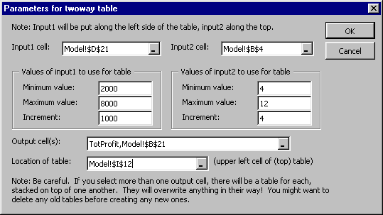
Creating a two-way table
To create a two-way table, go through the same steps as above for a one-way
table, but check the two-way option in Figure 2. Then the two-way dialog
box in Figure 5 appears. Here, we'll assume that both labor hour availability
(D21) and hourly wage rate (B4) are being varied, and we want to
keep track of the optimal profit and the number of labor hours used (B21).
(Any output cells can be selected.)

Figure 5
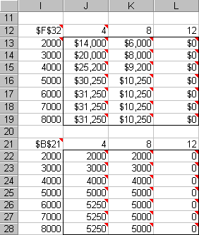
SolverTable then creates as many tables as there are output cells (in
a vertical direction), as shown in Figure 6. Note that each cell in a table
corresponds to a Solver run. For example, we see that when there are 4000
labor hours available and the wage rate is $4 per hour, the optimal profit
is $25,200 (top table) and all 4000 labor hours are used (bottom table).
Again, there are comments in selected cells. For example, the comments
in cells I13 and J12 remind you that the input cells are D11 and B4. The
comments in the body of each table report the Solver message, exactly as
with one-way tables.

Figure 6
As with all Solver models, it is a good idea to take a close look at
the answers and see whether they make sense. For example, in Figure 6 we
see all zeros in column L. Does this make sense? Yes, it probably does.
When the labor rate is $12 per hour and all other monetary inputs stay
constant, labor is evidently too expensive for the company to make a profit.
So it produces nothing!
Being creative
With some imagination, you can get SolverTable to run some really interesting
sensitivity analyses. For example, suppose we want to allow the availabilities
of all three resources (labor, metal, and glass) to change by common factor.
Then we need to change the model slightly, as indicated in Figure 7. Now
the original availabilities have been moved to column F, a change factor
has been inserted in column H, and formulas have been entered for
availabilities in column D. Specifically, the formula in cell D21 is =$H$21*F21,
which is then copied down.

Figure 7
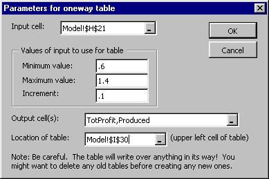
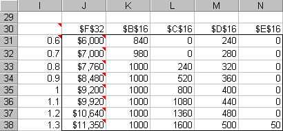
We can now do a one-way sensitivity analysis on this change factor,
using the settings in Figure 8. The corresponding table appears in Figure
9.

Figure 8

Figure 9
As another example, suppose you want to keep track of a function
of several cells in the model. For example, suppose you want to keep track
of the maximum number of frames of any single type produced, that is, the
maximum of the changing cell values. You can't select this as an output
directly because it doesn't appear anywhere in the model. But the
solution is simple: Create a formula for it in some unused cell, and then
specify this cell as an output cell.
SolverTable Difficulties
SolverTable relies on Solver. In fact, SolverTable invokes Solver for each
input value (or combination of input values). Therefore, all of the problems
that people have experienced with Solver are liable to occur with SolverTable.
However, we have tried to overcome one of Solver's more annoying features:
claiming that a model is not linear when we know it is linear. In
case you haven't run into this problem, we'll describe it first. When your
model is linear, you should check the Assume Linear Model box under Solver
Options. This has two advantages. First, it uses a faster algorithm (the
simplex method). Second, it is guaranteed (well, almost) to find the optimal
solution if an optimal solution exists. However, Solver uses its own rules
to check whether a model is linear. Because of numerical precision problems
inherent in computers, Solver sometimes decides that a model is not
linear, even though we know it is. In this case, it responds with an error
message that the conditions for a linear model are not satisfied.
SolverTable automatically checks for this error message. If Solver gives
it, then SolverTable reruns Solver (for this problem) with the Assume
Linear Model box unchecked and reports the result. However, to let
you know that all of this happened, the corresponding cells of the table
are colored yellow, and the comments in these cells describe the problem.
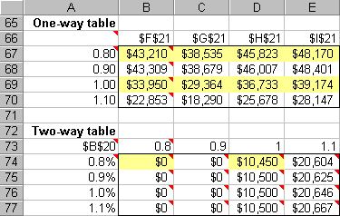
An example we encountered appears in Figure 10. This model is indeed linear.
However, when we formed the one-way table, Solver thought the model was
not linear for input values of 0.80 and 1.00, even though it agreed
that it was linear for input values of 0.90 and 1.10. Similarly, for the
two-way table, it thought the model was not linear for 2 of the 16 input
combinations. This is clearly strange behavior, but it happens fairly frequently.
At least, SolverTable provides a solution (using a nonlinear algorithm)
rather than the annoying "conditions for linear model are not satisfied"
Solver message.

Figure 10
